4. Juli 2018
Analysing Strava activities using Colab, Pandas & Matplotlib (Part 4)
 How do you analyse Strava activities—such as runs or bike rides—with Colab, Python, Pandas, and Matplotlib? In my fourth article on this topic, let’s invite scikit-learn and NLTK to the party, and apply some Machine Learning.
Let us find a problem that we can apply Machine Learning to at all cost─in order to demonstrate how to do Machine Learning with Colab, Pandas, Matplotlib, NLTK (Natural Language Toolkit), and scikit-learn. Here is the toy problem: which of my Strava activities were commutes?
Download Colab notebook
You can find the Colab notebook which I used for this article here:
File: Analysing_Strava_activities_using_Colab,_Pandas_and_Matplotlib_(Part_4).ipynb [44.63 kB]
Category:
Download: 1336
You can open this Colab notebook using Go to File>Upload Notebook… in Colab.
Do you need Machine Learning for that?
You don’t need Machine Learning to solve that problem. Simple heuristics would be sufficient here, such as looking at start location and end location of the route travelled, and then check whether these correspond to where I live (and have lived), and where I work and have worked. But let us use Machine Learning anyway, in order to demonstrate how to approach Machine Learning with Colab, Pandas, Matplotlib, NLTK, and scikit-learn. This is a problem where I have very good intuition and knowledge about; it is a fairly easy problem so we can focus on exploring the libraries; and I know perfectly how the data was generated, so the results are easy to interpret.
This article is not an introduction into Machine Learning. I expect that you know some concepts already. But you don’t have to be an expert either in order to follow what I write in this article. The fascinating thing is that Machine Learning no longer requires you to write enormous amounts of code─at least once you have processed your data into a format suitable for Machine Learning. We have already done that in the previous articles, see
- Analysing Strava activities using Colab, Pandas & Matplotlib: Part 1
- Analysing Strava activities using Colab, Pandas & Matplotlib: Part 2
- Analysing Strava activities using Colab, Pandas & Matplotlib: Part 3
Of course, not having to write code doesn’t mean that Machine Learning has become easy and can now be blindly applied. And it also doesn’t mean that you should apply Machine Learning to solve every problem coming your way. But remember, as I said, this is a learning project. Let us get on with it.
Understanding the domain
Strava is an app that allows users to record activities (in my case: runs, hikes, bicycle rides, ice-skating trips). Strava captures the distance travelled during that activity, the duration of the activity, the date of the activity, and also allows users to name each activity, and annotate each activity with whether it was a commute.
We are going to build a Machine Learning model that predicts whether a given activity was a commute. This is a supervised learning problem where we are able to train our model on labelled activities, and then can use this model to classify activities as commutes.
In the previous articles, we have already laid the groundwork: we explored the data, and we prepared the data. You don’t want to jump into applying ML without exploring the quality and nature of your data. But now we are in a good position.
Let us build a logistic regression model for classifying activities. A logistic regression model does not only predict labels but also provides an estimate on how certain the model is about its prediction. We will be able to look at the linear coefficients of the fitted regression model, and interpret what the model has learnt.
Splitting the data into test and training
As a canonical step in supervised learning, we split the data into training set and test set. I decided to use 80% of the data (314 activities) for training, and 20% of the data (79 activities) for testing.
import sklearn
from sklearn.model_selection import train_test_split
X = activities.reset_index()[['date', 'type', 'distance',
                              'elapsed_time', 'name']]
y = activities.reset_index()['commute']
X_train, X_test, y_train, y_test = (
    train_test_split(
        X, y,
        train_size=0.8,
        test_size=0.2,
        random_state=314,
        shuffle=True))
To build a classifier, we can use the date (including the time of the day), the type of activity (run, hike, ride, ice-skate), the duration, and the name of the activity.
X_train.sample(1).T
                                6
date          2014-07-07 07:31:59
type                          Run
distance                   4.9098
elapsed_time                 30.4
name              Morning Commute
Feature extraction
Let us get started with feature extraction (feature engineering). Extracting good features is an important step in Machine Learning. We will use our domain knowledge to construct useful feature for the logistic regression model we want to train.
What are good features for our model? The distance covered during the activity gives us a clue─my commute usually takes me along the same route. Duration gives us a clue─it usually takes me around the same time to commute. Time of the day gives us a clue─I usually commute in the mornings and sometimes in the evenings, but rarely in the middle of the day. The weekday gives us a clue─I don’t commute on weekends. Finally, I tend to give my commutes the same name.
As being said, start location and location would be very good points to start with but let us assume we do not have that data. Also while it would be a dream, I never ice-skate to work. Nor do I hike to work. But let us include that data anyway to make the problem slightly harder─and make sure the model still works once I actually start ice-skating to work. To make improvements, we should probably fit different models for each activity─the activity type (run, hike, bike ride) interacts with variables such as duration (I cycle faster than I run). But for now let us ignore that.
Weekend
I don’t commute on weekends. So we can construct a binary feature that captures whether an activity happened on a weekday or on the weekend. This is easy because Pandas has fairly decent support for handling dates; combine this with the apply function, the Swiss army knife in Pandas.
def weekend_features(X):
  is_weekend = lambda d: d.dayofweek >= 5
  weekend = X['date'].apply(is_weekend)
  return pd.get_dummies(weekend, prefix='weekend')
Here is a sample:
weekend_features(X_train).sample(5)
     weekend_False  weekend_True
224              1             0
57               1             0
295              1             0
259              0             1
315              0             1
NOTE: There is no point in including both weekend_True and weekend_False as dummy variables since the value of one completely predicts the other, and since weekend is already a binary (Boolean) variable. I originally used day of the week as a feature, for which we need dummy variables, and then forgot to remove the code that created dummy variables.
Time of day
Let us break the day into periods (“night”, “morning”, “late_morning”, “early_afternoon”, “late_afternoon”, “evening”, “late_evening”).
def time_features(X):
  time = pd.cut(X['date'].apply(lambda d: d.hour),
                     right=False,
                     bins=[0, 6, 9, 12, 15, 18, 21, 24],
                     labels=['night',
                             'morning',
                             'late_morning',
                             'early_afternoon',
                             'late_afternoon',
                             'evening',
                             'late_evening'])
  return pd.get_dummies(time, prefix='time')
Here is a sample (transposed in order to fit on this page):
time_features(X_train).sample(5).T
                     196  293  302  346  215
time_night              0    0    0    0    0
time_morning            1    0    0    0    1
time_late_morning       0    0    1    0    0
time_early_afternoon    0    1    0    0    0
time_late_afternoon     0    0    0    1    0
time_evening            0    0    0    0    0
time_late_evening       0    0    0    0    0
Distance
Let us build some distance-based features using domain knowledge─I ever run so far, I ever cycle so far, and my commutes tend to be in the shorter range. By setting the bin edges using a log scale, we have “higher resolution” (i.e. smaller bins) for short distances than for long distances.
def distance_features(X):
  distance = pd.cut(X['distance'],
                    bins=np.logspace(1, 7, base=2, num=10),
                    labels=['xxxs', 'xxs',
                            'xs', 's', 'm',
                            'l', 'xl', 'xxl', 'xxxl'])
  return pd.get_dummies(distance, prefix='distance')
Here is a sample (transposed in order to fit on this page):
distance_features(X_train).sample(5).T
               89   349  272  144  367
distance_xxxs    0    0    1    0    0
distance_xxs     0    0    0    1    0
distance_xs      0    0    0    0    0
distance_s       0    1    0    0    1
distance_m       0    0    0    0    0
distance_l       0    0    0    0    0
distance_xl      0    0    0    0    0
distance_xxl     1    0    0    0    0
distance_xxxl    0    0    0    0    0
Duration
Similar reasoning as for the distance of the activity.
def duration_features(X):
  duration = pd.cut(X['elapsed_time'],
                    bins=np.logspace(4, 8, base=2, num=10),
                    labels=['xxxs', 'xxs',
                            'xs', 's', 'm',
                            'l', 'xl', 'xxl', 'xxxl'])
  return pd.get_dummies(duration, prefix='duration')
Here is a sample (transposed in order to fit on this page):
duration_features(X_train).sample(5).T
               240  154  164  25   136
duration_xxxs    0    0    0    0    0
duration_xxs     1    0    0    1    0
duration_xs      0    0    1    0    1
duration_s       0    0    0    0    0
duration_m       0    0    0    0    0
duration_l       0    0    0    0    0
duration_xl      0    1    0    0    0
duration_xxl     0    0    0    0    0
duration_xxxl    0    0    0    0    0
Name
We start with the name of the activity. If I called an activity “Morning Commute”, I would like the model to learn that this is a commute. So how do we feed text information into our model? Fortunately, Pandas supports text processing, and works nicely together with the Natural Language Toolkit (NLTK).
So let us build features from the names of the activities.
- Normalize words by first taking the stem of the words, and then map the stem onto a meaningful word─NLTK does that for us.
- Drop short words because short words are often stop words such as “to” and we do not want the model to learn any association between stop words and the likelihood of whether activities are commutes. There are more sophisticated approaches, but this is simple.
- Drop words that don’t appear more than once in the whole set of activities because they won’t help us in the prediction (note that we are using information from the test set here─if we wanted to evaluate the model on unseen activities, this would not be advisable).
- Only keep words that appear in the training data.
- Perform some stunt with Pandas to get a binary feature for each word, indicating whether the word is present in the name of the activity.
I am not immensely proud of the following code, I had no time to look for a prettier solution. But it gets the job done.
def word_features(X, train_indices):
  lemmatizer = WordNetLemmatizer()
  lemmatize_words = lambda s: [lemmatizer.lemmatize(w) for w in s]
  # helpers
  word_separators = r'[,:()!? ]'
  word_hyphenators = r'[\-_]'
  remove_short_words = lambda s: list(filter(lambda w: len(w) >= 5, s))
  make_unique = lambda s: list(set(s))
  prefix_with_word = lambda s: ['word_' + w for w in s]
  # transform
  words = (
      X['name']
        .str.replace(word_separators, ' ')
        .str.replace(word_hyphenators, '')
        .str.lower()
        .str.split(' ')
        .apply(lambda s: [w.lower() for w in s])
        .apply(remove_short_words)
        .apply(make_unique)
        .apply(lemmatize_words)
        .apply(prefix_with_word)
        .apply(pd.Series)
        .stack()
        .reset_index(level=1, drop=True))
  # Pandas stunt
  words = words.reset_index().set_index(['index', 0])
  words['present'] = 1
  words = words.unstack(0, fill_value=0)
  words.columns.names = ['present', 'word']
  words.columns = words.columns.droplevel(level='present')
  # Correct for words only in test set; we could not possibly know
  # these words prior to prediction time.
  words_train = words.reindex(train_indices)
  words_only_in_test = (
      words_train.columns
          .to_series()
          .loc[words_train.sum() == 0]
          .index.values)
  words = words.drop(columns=words_only_in_test)
  return words
Note that we process both training set and test set at once here because we need to extract features from both. At the same time, we avoid keeping information derived from the test set (e.g. words that occur only in the test set). This is to avoid information from the test set does not leak into the training set.
This is a sample showing 3 out of 185 lemmatized words: vanguard, balcombe, and commute. See how the title of some of my activities actually gives away the fact that the activities are commutes! But not always does the title contain the word “commute”. Later, we will train models without lookoing at the words in the title.
word   word_vanguard  word_balcombe  word_commute
index
54                 0              0             1
51                 0              1             0
142                0              0             1
125                0              0             1
89                 0              0             0
Defining three different sets of features
In order to explore how many features we actually need in order to build a strong classifier, let us construct three different sets of features.
def features(X_features_list, train_index, test_index):
  X_features = pd.concat(X_features_list, axis=1).fillna(value=0)
  return (
      X_features.iloc[train_index],
      X_features.iloc[test_index]
  )
First, the distance_duration feature set which only contains the (binary) distance features and the duration features. The distance_duration feature set contains 18 features.
X_distance_duration_train, X_distance_duration_test = (
    features([
        distance_features(X),
        duration_features(X),
    ],
    X_train.index,
    X_test.index))
Second, the no_word feature set which only contains all features except the word features extracted from the name of the activities. These features do not contain any information about the name of the activity. The no_word feature set contains 31 features.
X_no_word_train, X_no_word_test = (
    features([
        type_features(X),
        weekend_features(X),
        time_features(X),
        distance_features(X),
        duration_features(X),
    ],
    X_train.index,
    X_test.index))
Third, the all feature set which contains all 216 features (185 word features and 31 other features). Given that we have only 314 training instances, we will have to avoid overfitting.
X_all_train, X_all_test = (
    features([
        type_features(X),
        weekend_features(X),
        time_features(X),
        distance_features(X),
        duration_features(X),
        word_features(X, X_train.index)
    ],
    X_train.index,
    X_test.index))
Usefulness of these features
We can already check whether these features are useful to classifiers. Pandas support for cross-tabulation can help us understand how informative the features are. For example
pd.crosstab(
    time_features(X_train).idxmax(axis=1),
    y_train,
    rownames=[''],
    colnames=['commute'])
commute          0    1
weekend_False   55  147
weekend_True   112    0
So this confirms clearly: no commutes on weekends.
pd.crosstab(
    distance_features(X_train).idxmax(axis=1),
    y_train,
    rownames=[''],
    colnames=['commute'])
commute         0   1
distance_l     21   0
distance_m     32   0
distance_s     40  48
distance_xl    20   0
distance_xs    23  49
distance_xxl    8   0
distance_xxs   11  49
distance_xxxl   5   0
distance_xxxs   7   1
It is clear that commutes only cover certain distances, but distance alone cannot
separate commutes from other activities.
Model fitting and model selection
We will build fifteen different models: five classifiers trained on three different sets of features. Why? Just out of curiosity, to see how they are doing. And to show how we can experiment with scikit-learn in Colab.
Baseline
As a very first thing, we train a “dummy” classifier. This is going to establish a baseline for all the other models. The training set is well-balanced and roughly half of the activities are commutes. So by configuring the DummyClassifier to always classify an activity as a commute (as this is the most frequent activity in the training set we sampled before), we get a baseline of 53% accuracy. Of course, we expect that we can improve on that dramatically.
from sklearn.dummy import DummyClassifier
dummy = DummyClassifier('most_frequent')
dummy.fit(X_all_train, y_train)
dummy.score(X_all_train, y_train)
Logistic Regression
Let us now train the logistic regression model. This is now relatively simple compared to all the hard work that went into feature extraction. Basically, training a model using scikit-learn works like this─not only for logistic regression:
model = LogisticRegression()
model.fit(X_features_train, y_train)
The fit method estimates the regression coefficients from the training set and the training labels.
Now we know how to fit models, let us also perform model selection in order to find a good regularization parameter C. We have up to 216 features for only 314 training examples, so we use regularization in the hope that this will counter-act overfitting.
from sklearn.linear_model import LogisticRegression
from sklearn.model_selection import GridSearchCV
def train_logistic_regression_model(X_features_train, y_train):
  lr_gs = GridSearchCV(LogisticRegression(random_state=99),
                           {'C': [0.01, 0.1, 1.0, 10, 100]},
                           scoring='roc_auc')
  lr_gs.fit(X_features_train, y_train)
  return lr_gs.best_estimator_, lr_gs.best_score_
With the scoring parameter, we specify the metric to optimize for. What metric to choose depends a little bit on the intended use of the model. We can choose e.g. to optimize for precision, for recall, for F1 score (a “balance” between precision and recall). Here, we chose the Area under the ROC curve.
I have set the random_state parameter for reproducibility of the results (for the purpose of including the results in this article).
Other classifiers
Let’s add four more classifiers:
In the code, this will look like:
def train_logistic_regression_model(X_features_train, y_train):
    ...
def train_naive_bayes_model(X_features_train, y_train):
    ...
def train_support_vector_machine(X_features_train, y_train):
    ...
def train_knn_classifier(X_features_train, y_train):
    ...
def train_decision_tree(X_features_train, y_train):
    ...
I won’t go into any detail here. But note that the binary features work with all these classifiers out-of-the-box. However, remember that we built the features for the logistic regression model, not e.g. for the decision tree which actually does not actually require binary features.
Actual training
Up to now, we have defined functions that allow us to train models on different feature sets. What remains is that we actually call these functions in order to train the fifteen different models. Five different types of classifiers:
training_functions = {
  'Logistic Regression': train_logistic_regression_model,
  'Naive Bayes': train_naive_bayes_model,
  'Support Vector Machine': train_support_vector_machine,
  'K-Nearest Neighbors': train_knn_classifier,
  'Decision Tree': train_decision_tree,
}
And three different feature sets:
features_train = {
   'distance_duration': X_distance_duration_train,
   'no_word': X_no_word_train,
   'all': X_all_train,
}
Train all fifteen models:
models = []
for c, f in training_functions.items():
  for d, x in features_train.items():
    m_n = '%s_%s' % (c, d)
    print('Training classifier "%s" with features "%s"...' % (c, d))
    m, _ = f(x, y_train)
    models.append({
        'classifier': c,
        'features': d,
        'model': m,
    })
We are now ready to evaluate how the model performs on the test set. Note that we never looked at the performance of the test set until now in order not to spoil the estimate for how well the models generalize to unseen data.
Evaluation
Performance on test set
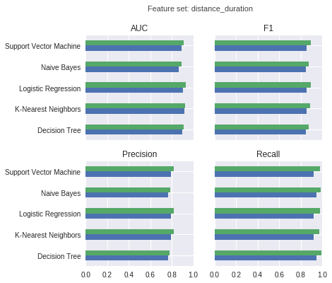
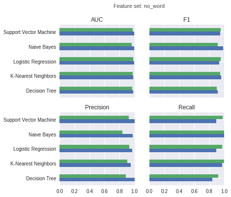
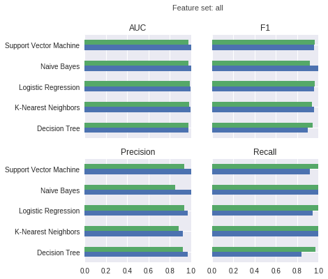
The following charts show training performance (green) and test performance (blue) with regard to AUC (area under ROC curve), F1 score, precision, and recall.
For the models trained on distance features and duration features only:
For the models trained on all features except the word features derived from the names of the activities:
For the models trained on all features:
Receiver Operating Characteristic (ROC)
If you have a smoke alarm, then you would like its detector to alarm you every time there is a fire (let’s ignore other sources of smoke for the sake of the discussion) in your apartment; you want your smoke alarm to have near 100% recall. Recall (also called sensitivity or true positive rate) describes how likely the smoke alarm goes off when there actually is a fire. At the same time, you do not want your smoke alarm to go off when there is not a fire. Thus you want your smoke alarm to have a low false alarm rate (also called fall-out or false positive rate).
We usually need to make a trade-off between a high true positive rate and a low false positive rate. In the example of the smoke alarm, we might accept the occasional false alarm when cooking if that also increases the chance of the smoke alarm detecting an actual fire.
With the logistic regression model, we can actually make this trade-off by selecting an appropriate threshold on the predicted confidence scores. The less likely we want to mistakenly classify an activity as a commute, the higher we set the threshold. In the Strava example, the true positive rate captures how likely is that the model correctly detects a commute as such the false positive rate describes how likely is it that the model classifies a non-commute as a commute.
The ROC curve plots the true positive rate against the false positive rate for decreasing thresholds. For a sufficiently high threshold, the logistic regression model will classifies all activities as non-commutes: hence we have 0% false positive rate but also 0% true positive rate. At the other extreme─with a sufficiently low threshold─the logistic regression model classifies all activities as commutes and trivially achieves 100% true positive rate but also 100% false positive rate. Better trade-offs are to be found for threshold values in between. A perfect classifier achieves 100% true positive rate and 0% false positive rate─this ends up as at coordinates (0, 1) in the top-left corner of the graph.
For the logistic regression models (left) and the support vector machines (right), these are the ROC curves evaluated on the test set:
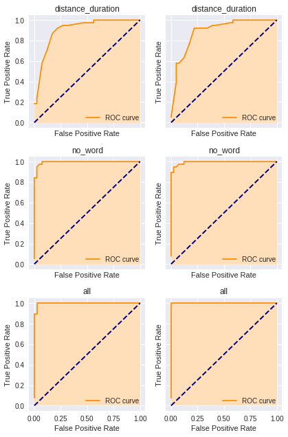
We can see that the area under the curve is larger for the models trained on all features than the models trained on distance and duration features only. While the support vector machine achieves an AUC of 1, it does not have 100% recall─this implies we do not use the optimal threshold for the support vector machine with respect to the test set.
Interpreting coefficients
We can look at the regression coefficients of the logistic regression models. For example, let us look at the model we trained on the no_word feature set:
coef = pd.Series(models_df.loc[('Logistic Regression', 'no_word'), 'model'].coef_[0], index=X_no_word_train.columns)
print('\nPositive:')
print(coef.loc[coef > 0].sort_values(ascending=False))
print('\nNegative:')
print(coef.loc[coef < 0].sort_values(ascending=True))
This shows that certain duration/distance and time of the day are making it more likely that an activity is a commute (morning, short distance) whereas activities on weekends and activities with long duration make it less likely.
Positive:
duration_xxxs          3.274838
duration_xxs           3.205310
duration_xs            2.601083
distance_s             2.513659
time_morning           1.780568
duration_s             1.667919
...
Negative:
weekend_True           -3.894452
duration_m             -3.839719
time_late_evening      -2.717444
duration_l             -2.431965
distance_xxxl          -2.426155
distance_xxl           -2.156228
...
Conclusion
In this article series, I have demonstrated how to use Colab, Pandas & Matplotlib, as well as NLTK and scikit-learn in order to interactively explore data, visualize data, transform data, and apply Machine Learning. I have included the Colab (IPython) notebooks. I hope the tutorial inspires you. I’m not finished here─I have still much too learn.